Smart Parking – IoT Perspectives
13 December 202121 September 2017 | Software
The pioneering of smart parking
Using the disturbance of the Earth’s magnetic field to detect the presence of a vehicle is not a new concept. More than five decades ago, Koerner and Brickner imagined a system where this kind of information can be obtained, centralized and processed. Two use cases of the pioneers in this field, namely parking management and traffic control, appeared to have a high potential and be adopted on a large scale.
Considering that the number of cars was 10 times smaller at that time, the attempts of establishing the technical means for getting traffic information were in the early stages. Knowing the limitations which the geomagnetic transducers had in the ‘60s and ‘70s, it becomes clear why equipping too many parking slots with such detectors was not an option.
The phenomenon is illustrated in the following figure, considering that the sensor is placed where the field changes are largest.
Ferrous object + Uniform geomagnetic field = Distorted geomagnetic field
The shape of the distorted lines depends on the geometry and the ferrous composition of the vehicle, each car model determining a unique magnetic fingerprint. The larger the set of measurements, the better the accuracy of detection will be. The place with the largest amount of metal is near the engine block, and there is no guarantee that all cars will park identically.
Therefore, the chosen place for mounting the sensor is in the center of the parking slot. It can be partially buried or simply fixed on the ground when the height is not an obstacle. A sensor serves just one parking slot, the delivered information being either “free” or “occupied”. To do so, the detection algorithm must be immune to the presence of other cars in the nearby. The terminals are similar in size and shape to a small mole-hill.
Click here to watch a short film describing the proof of concept.
How it works?
By setting the reliable vehicle detection as the key feature of the device, we can analyze the type of signals and their range of interest. The magnetic field measurable on Earth can take values in an extremely broad range, covering 17 orders of magnitude. For example, the human brain magnetic field is around 10-13 T, while the peak values generated in a controlled environment, by the Z machine at SNL, are around 104 T.
The measurement principle and the constructive type differs from one case to the other. The magnetic field of the planet itself takes values between 22 and 66 µT, when measured on the surface. Eliminating the areas covered by water, and narrowing further this range by considering only the populated zones, the range mentioned above is diminished by 10%.
Two capital cities are worth mentioning for the extremes in this respect: Asuncion, Paraguay – for 22.2 µT, and Hobart, Tasmania for 61.9 µT. The total values measurable in Romania are between 47.4 and 50.0 µT, just 5.9% from the entire worldwide range.
The total value is the result of the North-South, East-West, and down-up components. All of them have small changes in time, the absolute values of the typical rates being 1…100 nT/year. The table below contains these values for Cluj-Napoca, as of 2017.
| Component | Geomagnetic field [µT] | Change rate [nT/yr] |
|---|---|---|
| N-S | 21.4 | 1.5 |
| E-W | 2.0 | 42.7 |
| down-up | 43.8 | 35.0 |
| Total | 48.8 | 33.8 |
The change rates are 1000 times smaller than the values of interest to be measured, below the 1-LSB resolution. The RMS noise is covering them, especially during low-power operation modes. That’s why the change rates for any component, even if focusing on multiple years, are barely detectable using commercial geomagnetic sensors.
If one design criterion is long battery-life, the low-power mode should be considered for all components supporting it, but this leads to a slightly noisy operation. Fortunately, the change rates are negligible and do not influence the required accuracy for detecting the presence of a vehicle.
By analyzing measurements of the distortions generated by an automobile to the Earth’s magnetic field, two immediate conclusions can be depicted. Firstly, one may observe that they can be smaller if compared to the differences given just by changing the location. In short, this means that a detection system designed to use the absolute values will not operate properly when moved to another geographic area. Secondly, most of the sensing values have the same magnitude order as the worldwide geomagnetic field.
To overcome the location issue, one may think of adding extra information such as coordinates, altitude, and look-up tables, but this may not be always feasible due to computing and storage restraints. Even if a few bytes of ROM can be added to the system, the stored content needs to be extremely accurate, based on an absolute measurement performed in that place. Maybe the most critical aspect is that these values are varying in time.
A more flexible approach would be to use relative values, based on offsets given by a self-nulling operation. In this way, the detector can operate properly everywhere in the world, subtracting for each measurement the information characteristic to that specific location. Using this approach, the offsets will contain also the local non-geographic information, such as magnetization of the soil, surroundings etc. This is of particular interest when placing the same type of detector on different surfaces, such as concrete, cement, metal, or plain soil. After all, we are interested only in detecting the arrival and departure of vehicles, separate from all other influences. A higher level of flexibility can be achieved when such a self-nulling can be performed on-demand, using a wireless network. This can be done based on a fixed period – e.g. 6 to 12 months, or when the read data is suspected to be no longer accurate.
Smart vehicle detection from the embedded perspective
We can find over 14 vendors for integrated geomagnetic sensors and, by knowing the design criteria of a specific device, the best one can be filtered out by comparing their key parameters. Among them, one may consider the 3.3 V operation, industrial temperature range, high sensitivity, low current, I2C or/and SPI bus interfaces, self-test capability etc.
The figure below illustrates the current consumption of such a sensor versus the number of readings per second. In power-down mode, it requires less than 1 µA, is of triaxial type, uses the I2C bus and comes in a VFLGA package of 2x2x1 mm.
If sensing the magnetic field can be seen as the heart of the device, then all operations need to be supervised by a brain. The Atmel picoPower family of 8-bit AVR microcontrollers was considered in this respect. It achieves throughputs around 1 MIPS per MHz, the target platform running at 3.3 V and 8 MHz. It can respond to a combination of specific restrictions: capable of long-time battery operation, good balance between resources and computing power, power-down capabilities, industrial temperature range, programmable digital IOs, I2C and UART interfaces, high-level programming support, self-programmable flash memory, and many others. Projects can be developed using Atmel Studio, Atmel AVR8 GNU toolchain, WinAVR, Labcenter Proteus, or Arduino IDE.
The code of the project is written entirely in C++.
The ATmega328P chip is consuming only 0.1 µA in power-down mode, and 3.2 mA in active mode for the specified configuration. An overview of the terminal and its belonging modules is given below.
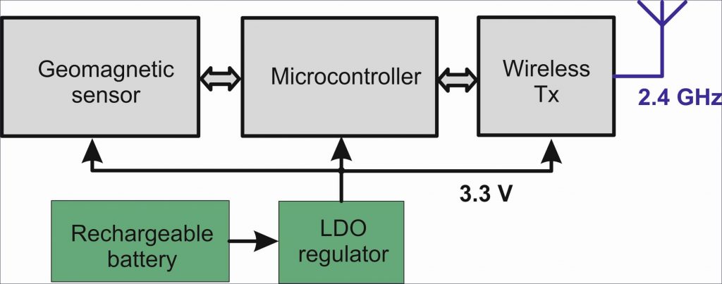 The terminal is powered by a rechargeable battery, which may consist of 3 to 5 cells of 18650 type. The voltage usually differs after various recharging phases, the role of the low-dropout voltage regulator being to assure that all three chips – sensor, microcontroller and wireless – are always operating at a stabilized voltage of 3.3 V. If the maximum allowed voltage for the mentioned chips is around 3.6 V, then a fully charged battery pack will damage the components if connected directly. A key parameter of the regulator is the dropout value as a function of temperature, as in the following picture.
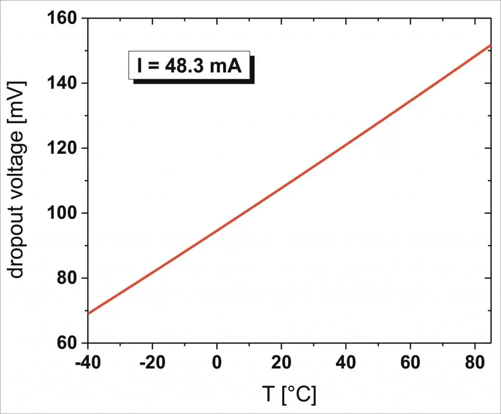
In this plot, 48.3 mA is the maximum current drawn by all circuits in active mode, the IEEE 802.15.4 wireless module having the largest contribution to this value. Using a power of 8 dBm, it can send data at a maximum indoor range of 60 m. If the transmitter is under a vehicle – which is the case of an occupied slot – this range is reduced due to the massive metallic shielding. The power-down current consumption of the considered transmitter module is less than 3 µA.
It can be observed that at room temperature the dropout is around 100 mV, meaning that a battery of 3.4 V can still drive the circuits. When the required current is close to the lowest possible value – everything set to power-down mode – the dropout voltage decreases to less than 10 mV.
Because one design goal for the terminal is a long battery lifetime, determining fewer direct human interventions to it, let us consider a couple of simple examples for the current budget. The worst-case for the power supply would be running constantly in active mode, with no power-down at all. If the battery capacity is 10 Ah it will be drained in eight days and a half. If everything can be set to power-down mode without interruption, using the same logic for calculating the battery lifetime will lead to unrealistic durations; large temperature variations between seasons will shorten the battery lifetime quicker than the total current of approximately 4.1 µA.
If the battery lifetime goal is set to three years, the resulting current budget per hour will be around 380 µA, allowing to run everything in active mode 28 seconds out of one hour. In fact, this duration is even shorter, due to the power-down switch control imposed by the microcontroller. Having such estimations is of critical interest because the upper limitation for the number of transmitted packets needs to be correlated with the number of vehicle arrival and departure events.
IoT software development perspectives – smart cities
The flexibility provided by the IEEE 802.15.4 standard for configuring a personal wireless network is near-optimal for geometries like parking places, where unforeseen obstacles may shorten practical communication ranges between two fixed points. Adding intermediary transceivers – called routers in the ZigBee terminology – may help a lot if unsure about the reliability of a connection, though functional in ideal conditions. The terminal placed on the parking slot’s ground has a dedicated type of wireless unit, called end-device in the ZigBee terminology. There must be exactly one device with the role of setting up the network and receiving all the data, called coordinator. From a service-oriented perspective, it centralizes and processes all data, having also the possibility to write real-time information to a server.
Combining embedded engineering with big data solutions, the path towards smart cities is open by providing extended services, on a much larger scale. Online parking monitoring and reservation, intelligent indoor routing towards a specific parking place, metropolitan traffic management are only a few possible applications.
About the Author

Mihai


